Credit / Debit-Card Transaction Panels

Data Overview

Consumer-transaction panels aggregate millions of anonymized credit- and debit-card swipes from banks, processors, and fintech apps into a time-stamped ledger of where, when, and how much people spend. Vendors such as Facteus, Earnest Research, Second Measure, and Yodlee license this exhaust because it offers a near-real-time revenue telescope: when 32 % of U.S. payments flow through credit cards and 30 % through debit cards, the swipe tape becomes a statistically powerful proxy for company sales several weeks before earnings releases. Alpha persists because credit card data provides a more timely and direct proxy for company revenue than financial statements or consensus estimates, especially in retail and consumer sectors.

This project aims to segment customers of a retail brand based on their transaction behavior, using KMeans and KNN on engineered features derived from raw transaction data. The segmentation is performed quarterly, allowing for time-based analysis of customer behavior and segment share evolution.

Data Sources

Raw Transactions:
CSV/JSON file containing at least the following columns/keys (see image above):
- cardholder_id
- transaction_date
- amount
- etc.

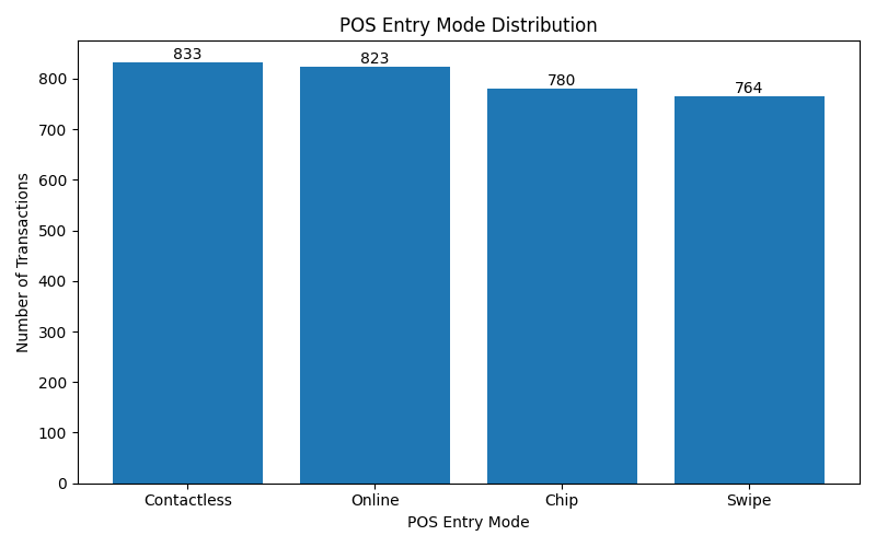
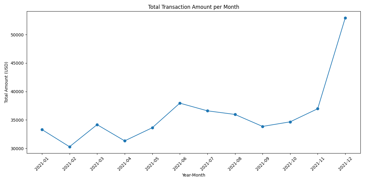
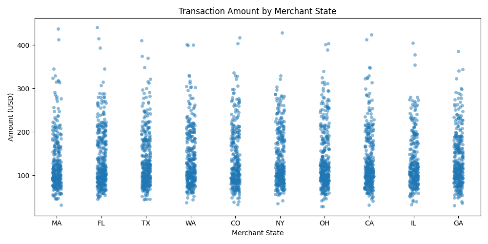
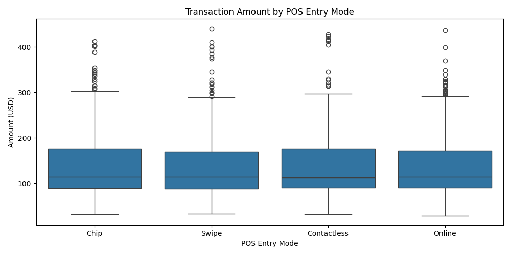
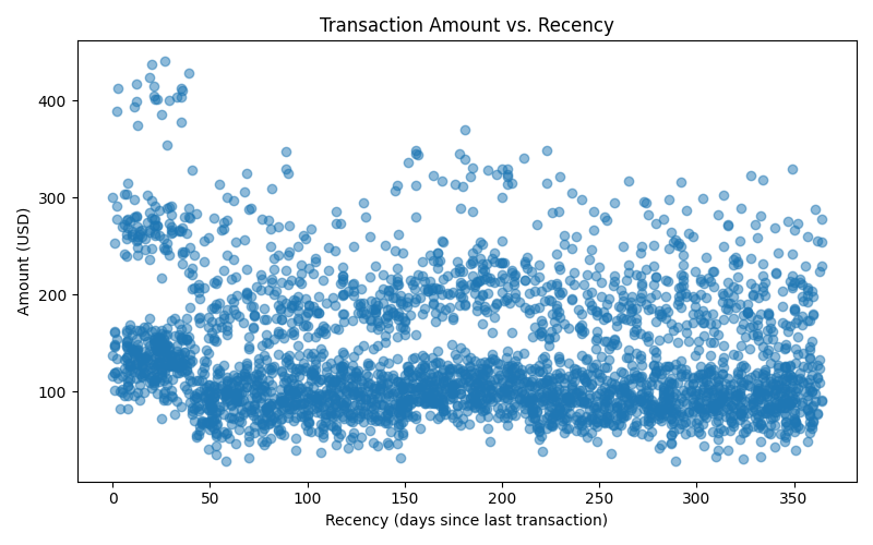
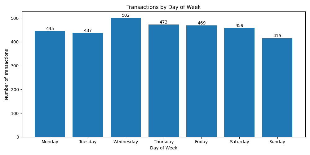
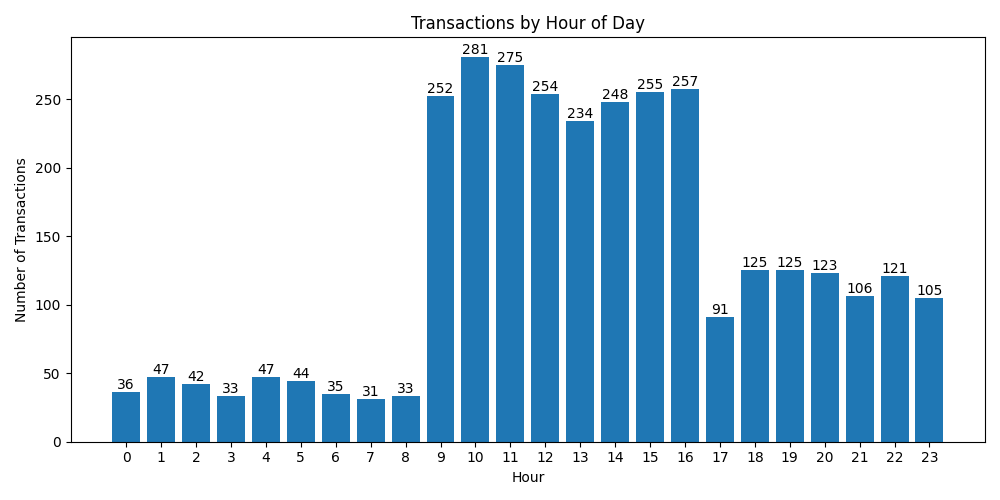
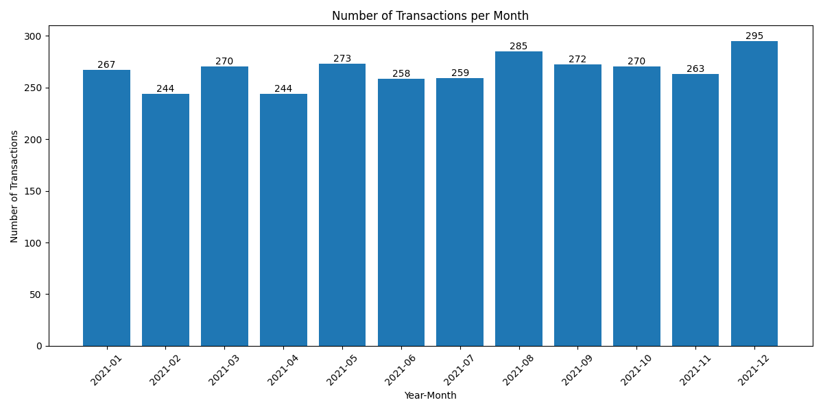
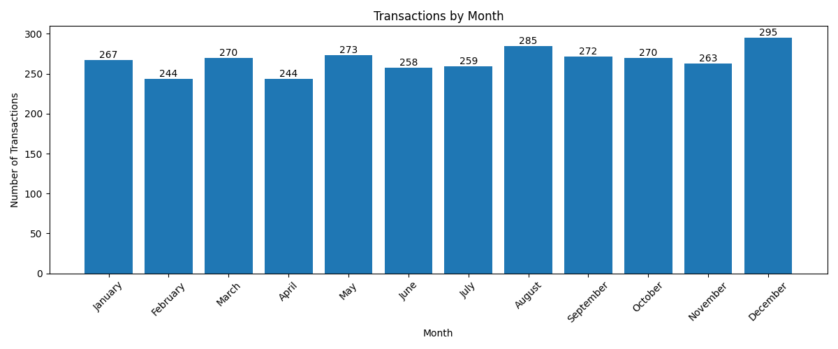
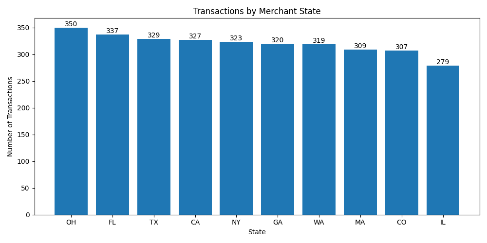
Exploratory Data Analysis

Data Processing Pipeline

KMeans:

Unsupervised clustering that finds k centroids to minimize within-cluster variance.
Great for discovering structure in historical data without labels.
Each customer is assigned to the nearest centroid (hard assignment).
Used to define the 5 customer segments
Limitation:
- Only gives hard assignments → each user belongs to one segment, even if they’re borderline.
- Assumes clusters are roughly spherical around a centroid (may not hold in real credit-card data).
- Not adaptive for new users unless you re-run the clustering.

KNN:

Supervised algorithm — requires labeled data.
In this case, labels come from the KMeans cluster assignments.
For a new user, looks at the k most similar historical users and assigns a probability distribution over clusters based on neighbor counts (or weighted by distance); e.g., Dormant 30%, Off-Season 25%, Holiday 45%.
Limitation:
- KNN is computationally heavier at inference (distance to all points).
- Requires a well-engineered feature space (recency, spend, frequency, etc.) to be meaningful.
- Doesn’t define new segments, only classifies into existing ones.

K-MEANS

1. Data Loading & Preparation

Read raw transaction data into a pandas DataFrame.
Convert transaction_date to datetime format.
Assign each transaction to a calendar quarter using pandas’ .dt.to_period('Q').

2. Feature Engineering (Quarterly)

For each quarter, compute customer-level features:

Recency: Days since last transaction (relative to the end of the quarter).
Frequency (last 7 days): Number of transactions in the last 7 days of the quarter.
Average Transaction Amount: Mean spend per transaction for the quarter.
Rolling 7-Day Spend: Total spend in the most recent 7-day window for each customer.
Seasonality Flags:
- Holiday Spend Flag: 1 if customer spent more in Nov/Dec than other months.
- Spring/Summer Spend Flag: 1 if customer spent more in Apr–Aug than other months.

All features are aligned so every customer in the quarter has a value for each feature (missing values filled with zero).

3. Quarterly Feature Aggregation

Features for all customers in all quarters are concatenated into a single DataFrame for clustering.

4. Clustering

Standardize features (optional, but recommended for KMeans).
Fit a KMeans model (used elbow method to determine 5 clusters) on all customer-quarter feature rows.
Assign each customer in each quarter to a segment.

The **largest drop in inertia** occurs before k = 5.

5. Segment Share Calculation

For each quarter, calculate the share of customers in each segment.
Output is a DataFrame: one row per quarter, columns for segment shares.

6. Output

The final output is a quarterly segment share table, suitable for time series analysis, modeling, or business reporting.
The trained KMeans model is also returned for future prediction or interpretation.

**Row 0 → 2021Q1**
0.302 for segment **0 (Dormant Low Spenders)**
→ ~30.2% of all customers in Q1 2021 were long-inactive, low spenders.
0.111 for segment **1 (Spring/Summer Loyalists)**
→ ~11.1% of customers were seasonal Q2/Q3 buyers — in Q1 they might be dormant waiting for warmer months.
0.206 for segment **2 (Off-Season Buyers)**
→ ~20.6% were steady buyers outside seasonal peaks.
0.030 for segment **3 (Engaged Holiday Shoppers)**
→ ~3.0% were high-frequency shoppers during holiday seasons — low here because Q1 is post-holiday.
0.351 for segment **4 (Holiday Champions)**
→ ~35.1% were high-value spenders with most purchases concentrated in Nov/Dec

If over time you see, for example:

pct_holiday_champions climbing in Q4 → likely strong holiday quarter revenue.
pct_dormant_low_spenders growing quarter-over-quarter → signals potential slowdown.
pct_spring_summer_loyalists peaking in Q2/Q3 → supports seasonal uplift forecast.

KNN

1. Why KNN?

The clusters (Dormant, Holiday Champions, etc.) were learned with KMeans.
But when a new customer comes in with engineered features (recency, frequency_7d, rolling_7d_spend, etc.), KMeans by itself just gives a hard assignment → "this customer belongs to cluster 2".
Sometimes we prefer soft probabilities → e.g.,
```
Dormant: 10%  
Spring/Summer Loyalist: 5%  
Off-Season Buyers: 30%  
Engaged Holiday Shoppers: 15%  
Holiday Champions: 40%
```
This is more useful for downstream models, because probabilities can be aggregated into segment shares more smoothly.

2. How KNN Helps

KNN classifier can estimate posterior probabilities by looking at the cluster labels of nearest neighbors:
- Count how many of the k neighbors belong to each cluster.
- Normalize counts into probabilities.
Example with k=10:
- 4 neighbors are cluster 0, 2 are cluster 2, 4 are cluster 4
- Probabilities = [0.4, 0, 0.2, 0, 0.4].

3. Why not just use KMeans distances?
You can compute soft assignments using the inverse distance to centroids. But KNN is often more robust to irregular cluster shapes and doesn’t assume spherical geometry.

Application:
- For each quarter, instead of hard-counting “how many customers are in Cluster 3”, you average their probability mass.
- This gives a smoother quarterly segment share time series, less noisy than hard cluster counts.
- Those smoothed shares become predictors in your Lululemon revenue regression.

REVENUE PREDICTION

Historical discovery: Run KMeans on 2016–2020 data → define the 5 customer segments.
Train KNN: Fit KNN using KMeans labels as “truth”.
Each quarter:
- Assign new customers using KNN → get soft probabilities.
- Aggregate to quarterly segment share probabilities.
- Merge with historical revenue.
Regression modeling: Use segment shares (from KNN) as predictors of LULU revenue → derive trading signals (compare model vs. consensus).

PCA for Visualization

Segment 0: Dormant/Low Spenders
Segment 1: Spring/Summer Loyalists
Segment 2: Off-Season Buyers
Segment 3: Engaged Holiday Shoppers
Segment 4: Holiday Champions

PCA1 is usually loaded most heavily on **recent spend (rolling_7d_spend, recency_days, frequency_7d, avg_transaction_amount)**, so clusters along this axis separate by engagement and recent spend intensity.
PCA2 may pick up on **seasonality (holiday or spring/summer flags)**, so clusters split up/down by when in the year they spend.

Next Steps

Merge with historical revenue (and possibly other drivers like macroeconomic data, Google Trends, weather, etc.).
Feature selection – not every column will have alpha; test which segment share changes correlate with future revenue beats/misses.
Feature Expansion – add more behavioral, geographic, or product-level features.
Model Comparison – try other clustering algorithms (e.g., DBSCAN, hierarchical).
Model fitting – train regression or time-series models on multiple years of quarterly data.
Validation & backtesting – check if the model would have predicted past revenue surprises and if those predictions would have generated profitable trades.
With more historical transaction data:
- Re-run the transaction-to-segment pipeline for every available year in the credit card dataset.
- Keep the same KMeans clustering model (or retrain on the entire multi-year dataset, but don’t change it per year).
- Append each quarter’s segment shares to build a multi-year quarterly table (ideally 3–5 years, i.e., 12–20 quarters).
Once you have a historical baseline:
- Every quarter end (T+1 week): run the pipeline to generate that quarter’s segment shares.
- Append the row to your historical table so the model stays updated.
- The new quarter’s values feed into your pre-earnings prediction.
If you want mid-quarter forecasts:
- Run it monthly or weekly to get early signals about how the quarter is trending.
- Extrapolate partial-quarter numbers to a full-quarter projection.

Entire Flow

Historical build: OnceCreate long history for training & backtesting
Quarterly update: After each quarter closes, add the most recent quarter for re-training
Pre-earnings run: ~1 week before earningsFeed current quarter’s segment shares into the model to predict revenue vs. consensus
Signal handoff: After model outputPass alpha signal to PM/trading team for position sizing

Reflections and Insights

Strengths

Temporal Segmentation: Quarterly analysis captures seasonal and promotional effects.
Feature Engineering: Carefully chosen features reflect recency, frequency, spend, and seasonality.
Scalable: Pipeline can be adapted for other merchants or time windows.

Limitations

Feature Set: Only basic features are used; richer data (e.g., product, location, payment type) could improve segmentation.
Cluster Interpretability: KMeans clusters are not labeled; interpretation requires post-hoc analysis.
Data Quality: Missing or noisy transaction data can affect feature accuracy.

Opportunities

Modeling: Segment shares can be used as features in forecasting or marketing models.
Trend Analysis: Track how segment shares evolve over time to inform strategy.

Reference